You heard that right, “COOL” ways to use Excel conditional formatting. Since this is an accounting blog, I figured we can all be open about the fact that most of us get way too much enjoyment out learning new Excel tricks. I’m guilty of it myself.
But, I wasn’t always this way.
When I started at PwC, my Excel skills were not up to par with the rest of the team. Terms like, Vlookups, Pivot Tables, and Conditional formatting would be thrown around the audit room with the expectation that I had some clue as to what they were talking about. Nope.
However, my senior acknowledged my lack of Excel skills and told me to start researching certain Excel features to get me up to speed. One of them was called “Conditional Formatting”.
To help kickstart your accounting career, I figured it’s time to dive into the top 6 conditional formatting tricks I wish I knew when I started my first accounting job.
Here they are:
1) Duplicate Values
If you are staring at a long Excel column, and need to figure out which entries are duplicated, there is super simple way to knock this out. Check it out in the video below.
2) Greater Than, Less than, or Equal To Highlights
Need to figure out which values are greater than >$100? What about the cells that fall within <$90 – $100>? This can be done all by utilizing the Highlight Cells Rules.
If you already know this check, watch the first few seconds of the below video. There’s a floating instructor…No joke!
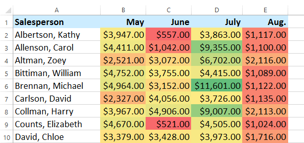
3) Color Coat Your Cells
Let’s say you want to display your spreadsheet based off of a pattern of particular values. I used this trick in my PBC lists that I would send to clients. For the PBC items that were not completed, the status showed up in Red. If it was pending information, the cell automatically displayed as Yellow and finally, if I received the item with no issues, a green cell would appear.
Pretty cool right? Again, super geeky Excel guy here.
4) Perform A Side-By-Side Comparison Of 2 Excel Lists
This is a great way to identify differences in lists, quickly. For example, if you have column 1 listing the names in Company A, and column 2 listing the names in Company B, and you want to compare the lists to see who is not included in either list, you can perform a side by side comparison using conditional formatting.
For a more detailed description of the capabilities, see the below video:
5) Highlight Certain Rows With Conditional Formatting
Have you ever had to highlight certain rows that contained a parameter (I.e. greater than, includes a certain word, etc?). Well, instead of having to highlight by hand, or sort the column, then highlight, then hope to set the spreadsheet back to it’s original form, instead you can use conditional formatting to automatically highlight rows based off of your specified criteria.
Here’s how to do it:
6) Super Advanced Row and Column Intersections by Multiple Criterion
Alright, this last trick is for you super geeky Excel accountants who just want to show off to their senior. Instead of having me try and explain what is going on here, as I do believe this is way past my own Excel master skills, check out how to create multiple conditional formatting criterion, drop downs and row/column intersections based off of those criterion. Crazy, I know.
Did I miss a cool conditional formatting trick that you know of? Feel free to share your Excel Ninja Skills in the comments


Follow Us!